
Second Nature is a demo for the Amiga OCS platform by Desire and TTE. It was released at Revision 2026, taking first place in the Amiga demo competition. It requires 1MB total RAM and fits on a single 880k floppy disk.
The people involved this time were:
- Me (gigabates): Code, additional graphics
- Pellicus: Code
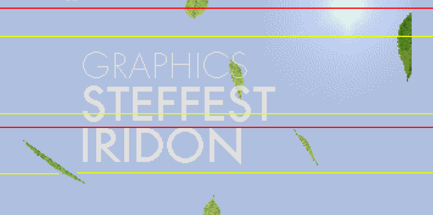
- Steffest: Graphics
- Iridon: Graphics
- H0ffman: Music, additional code
- RamonB5: Support
The concept #
I really wanted our next demo to have a coherent theme and narrative, rather than being a pure effects show (not that there’s anything wrong with those kind of demos). This is one thing that people seemed to like about Inside the Machine and I wanted to see if we could take that further as it’s maybe something that’s a little bit underexplored on OCS.
We’d floated the idea of a falling leaf effect for a previous demo, and it was something I’d been meaning to come back to, so I had a kind of vague nature theme in the back of my mind. I think any kind of realism tends to have an impact, as a lot of oldschool effects are quite abstract.
The other half of the concept came to me as I was out for a walk and saw a destroyed electronic organ abandoned by the canal. Aside from being a bit sad, it was interesting seeing how nature was already reclaiming it, with plants growing through its circuit boards. It was also quite jarring seeing something so out of place. This brought to mind themes around technology vs nature. From “Inside the Machine” to “The Machine Outside”, maybe?
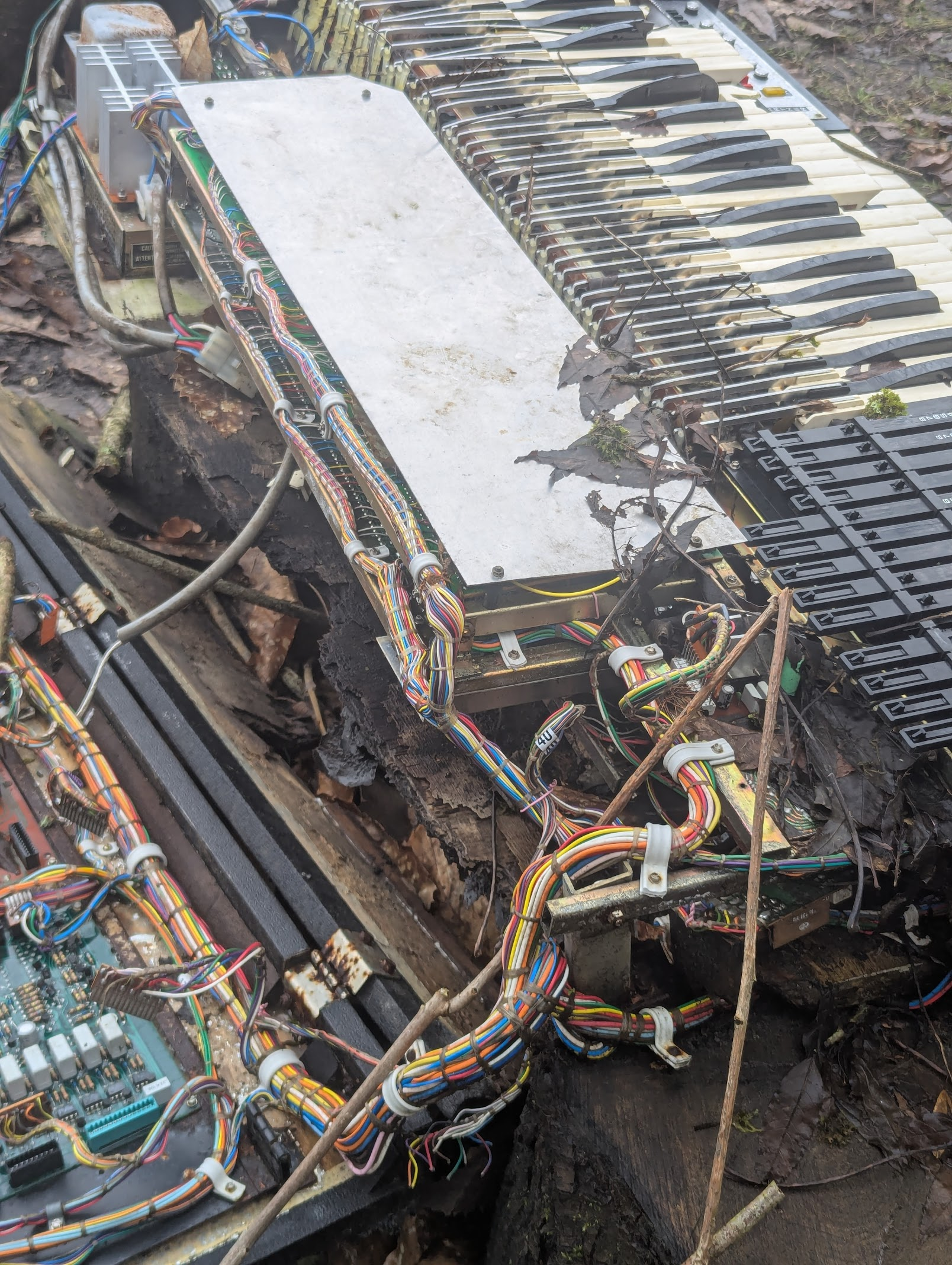
“organ donor”
In terms of effects, I really wanted to get away from blocky 4x4 or 8x8 chunky modes. I’d come up with a 1x1 c2p mode, and wanted to showcase this, but also wanted to include some non-chunky parts that use the chipset in other ways. Most importantly the effects had to actually fit the narrative.
Iridon had the great idea of splitting the demo into sections, based on time of day. Where originally the intention was to have a mixture of tech and nature elements throughout, having the tech come out at night worked really well to feature the glowing CRTs and lamps, and make it feel more mysterious.
The demo system #
On previous productions I’ve used Platon42’s awesome PlatOS demo framework, but this time round I wanted to try getting stuck into the details of making something more bespoke, catering to my own questionable preferences.
I started by thinking about what I like from other demo systems. I like the un-opinionated nature of Leonard’s LDOS. It allows you to include any hunk exe and only concerns itself with part loading and music. The clue is in the name, as it bills itself as a DOS, not an OS like PlatOS. This makes it possible to code parts using anything that can spit out an executable, including C/C++ which is something we wanted.
In general I prefer small reusable code over “do-everything” frameworks, bringing to mind the Unix philosophy of doing one thing well. This probably comes from my exposure to the JavaScript npm world, which I’m aware is not without its controversy. No pad-left or is-even though! This leads to some tradeoff of duplication vs persistent code and data. Having each part include its own copy of common logic has a cost.
I wanted to avoid runtime memory allocation inside the part executables for a few reasons:
- I generally write initial effect code outside of any framework, using BSS for memory. In the past this would require some rewriting to integrate into a demo.
- Keeping with the “generic exe” approach I wanted to avoid any kind of system calls
- Having dynamic memory allocations in code makes it much harder to do any static analysis, and derive the memory footprint of a given part. I wanted to be able to predict OOM situations at build time, which we’ll see later.
In fact just using BSS everywhere would actually be fine. LDOS explicitly recommends this, but it does have one downside. It needs to be cleared, which adds some overhead and may be unnecessary in some cases.
What I really wanted is a custom hunk/section type for uncleared BSS. I believe Eon does something like this. It would be possible to extend the hunk spec, and add a new header type, but I didn’t really want to add a dependency on a forked VASM to support this. As a workaround I fake it using a data hunk starting with a magic value. The disk builder detects this and treats it as uncleared BSS. I added nbss and nbss_c macros that make this look exactly like a regular section type in use.
nbss    macro
        section nbss,data
        dc.l    $deadbeef
        endm
           nbss
SomeData: ds.b 1024
PlatOS introduces the concept of loading vs preloading. Sometimes you don’t have space to have the current and next part fully loaded in memory, so you have the option to delay unpacking until execution, at the expense of a few frames delay. I decided to extend this concept in my implementation. I introduce an additional ‘deferred’ load strategy (naming things is hard!) where the data is unpacked, but BSS isn’t allocated / cleared, and relocations aren’t applied until execution. We can choose which of the three load strategies to use for each part based on the memory available.
The trackloader #
I decided to integrate h0ffman’s double buffered MFM trackloader, mainly because it looked cool, and the interrupt based approach fits well with the rest of the architecture which we’ll get onto. As it turned out this was quite experimental, and a lot less production ready than I thought, but luckily the man himself was around to battle harden it and make it much more resilient.
This has in-place ZX0 unpacking built in, which is great for load speed and memory usage. We used this method for all of the parts. Only the music data used an alternate approach of DEFLATE packing, which gave some significant gains in this case.
There’s probably a case to be made that the double buffering doesn’t bring enough benefit to justify the memory overhead, but it worked well for us in this instance.
Bootblock and file table #
The bootblock is fairly minimal. It locates the required memory blocks and loads and unpacks the file table and launcher program with zx0. Given the amount of free space in the bootblock, I made the decision to include the file table here. I would later come to regret this, but we did just about make it fit! This did require adding hunk merging into the disk builder to handle the large number of hunks output by GCC.
The file table format was initially based on the TTE disk format. Entries look like this:
| Offset | Size | Description |
|---|---|---|
| 0-7 | 8 | File ID (8 ASCII characters) |
| 8-11 | 4 | Disk location |
| 12-15 | 4 | Packed size with flags |
| 16-19 | 4 | File size (uncompressed size in bytes) |
The upper 10 bits of the packed size contain flags for the packing method, memory and hunk type, and a continuation flag, indicating whether there are additional hunks to load. Additional hunks follow as partial entries:
| Offset | Size | Description |
|---|---|---|
| 0-3 | 4 | Packed size with flags |
| 4-7 | 4 | File size (uncompressed size in bytes) |
Diskbuilder #
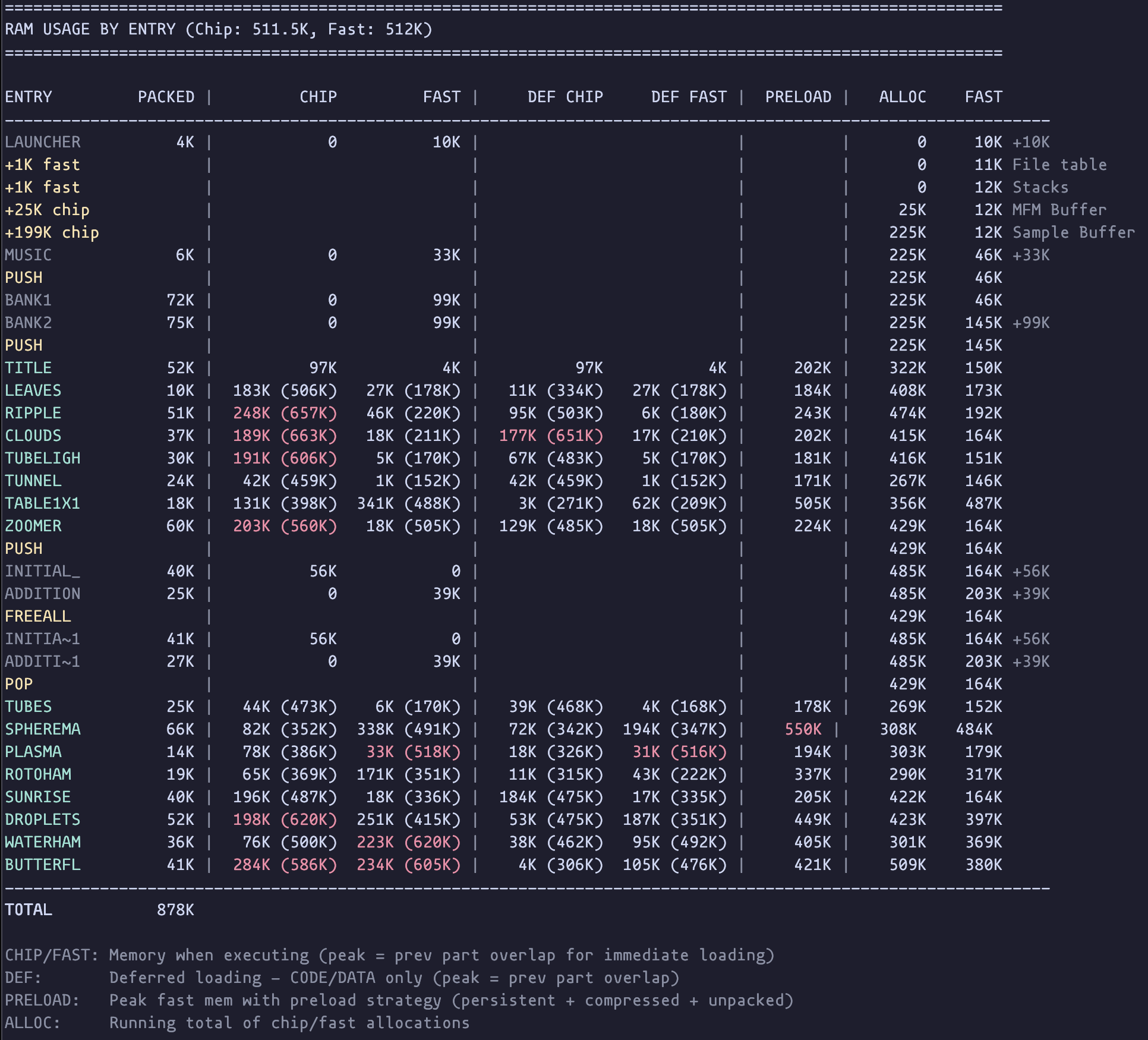
The ADF disk image is generated from a JSON layout file, listing the files and options. It generates a text summary, listing the memory footprint for each part when running, and when preloaded alongside the previous part using each potential strategy. This allows us to avoid runtime OOM conditions.
Interrupts #
I took a lot of inspiration from Hannibal’s excellent write-up of 3D Demo III. Massive thanks for this. I hadn’t previously appreciated the extent to which interrupt levels could be abused! I took the decision to run all effect code in interrupts using a pretty similar setup to the one he describes.
After initial setup, each part installs some interrupts and returns immediately, handing back control to the main launcher script, and running asynchronously. The launcher script is responsible for preloading the next part, and awaiting the frame when it should start, at which point the existing interrupts are uninstalled, and DMA etc is restored to a default state before executing the next part.
Personally I prefer this to the LDOS approach, where the current part is responsible for making system calls to load the next part, start/stop music etc. PlatOS’s approach to multitasking is more powerful, and doesn’t require the effect code to run in supervisor mode, allowing use of the a7 register, but overall I found that the interrupt approach met my needs and was easy to reason about.
H0ffman’s trackloader is also interrupt based, making it asynchronous and allowing us to do some background processing while data is loading.
Protothreads #
For the scripting in the demo, we used the protothreads pattern, that we originally learnt about from a talk by Trident/Fairlight. We used this on Vaporous, and it’s definitely going to be my preferred scripting solution from now on.
It allows you to write a routine that runs across a range of frames, and just write regular code separated by ‘wait for frame’ macros. You simply call this routine once a frame, and the entry and exit points are dynamically adjusted as the script progresses.
Script:
    SCRIPT_START

    SCRIPT_WAIT 200
    bsr SomeRoutine

    SCRIPT_WAIT 400
    move.w #100,SomeVar

    SCRIPT_END
    rts
SCRIPT_START jumps to the current entrypoint. SCRIPT_WAIT sets the entrypoint to that line, and exits if the current frame is less than the specified value.
SCRIPT_START macro
    move.l  ScriptPtr,-(sp) ; jump to current entrypoint
    rts
    endm

SCRIPT_WAIT macro
    move.l  #.\@check,ScriptPtr ; update entrypoint
.\@check:
    cmp.w   #\1,Frame
    bge.s   .\@next
    rts ; return from script if frame not reached
.\@next:
    endm

SCRIPT_END macro
    move.l  #.\@,ScriptPtr ; set entrypoint to end of script
.\@:
    endm
Amiga Convert #
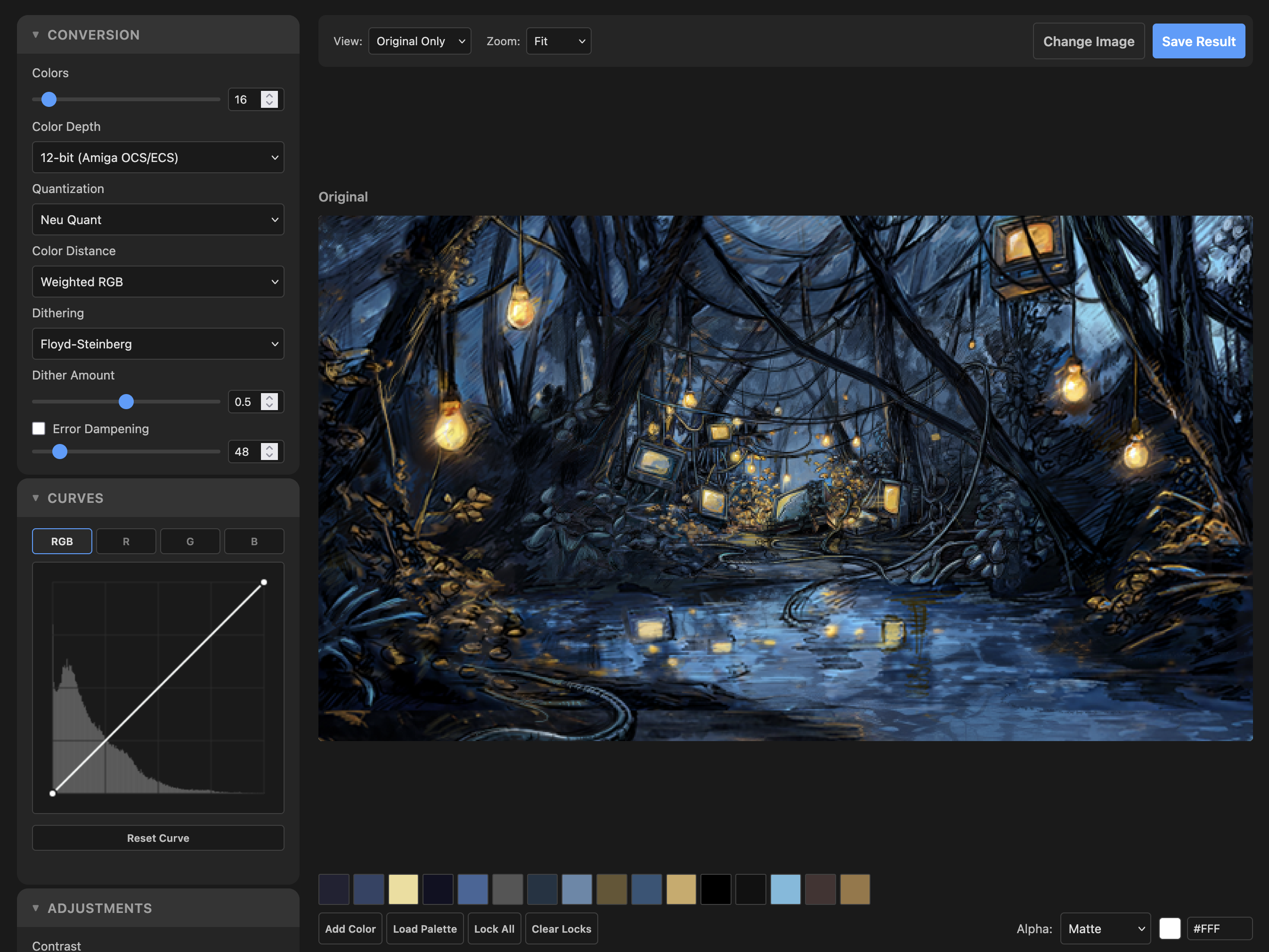
For better or worse, several of the graphics in this demo required some level of auto-conversion from full colour to Amiga 12bit RGB indexed modes. Having tried various options for this in the past, I finally got around to building a custom web based tool. It offers support for multiple dither modes, colour models and adjustments with a live preview. I’ve made this available online if you want to use it. https://amiga-convert.grahambates.com/
Chunky to Planar #
Several of the effects use a chunky to planar routine. This builds on the one used in previous productions, and as before it’s entirely blitter driven. The key new development is support for 1x1 resolution.
The great thing with using the blitter for this is that it can run in parallel with the CPU draw code. Especially with the increased resolution, we can c2p the buffer much faster than we can fill it. There are only so many moves you can fit in a frame. The focus of all the 1x1 effects in the demo is finding applications for this which don’t require us to fill an entire screen with pixels, as this would be far too slow.
There are a few variants of this routine used, but I’ll talk through the most complete version which is:
- 4 bitplanes
- 1x1 pixels
- one word per pixel
All the other variants are simplified versions of what I’m about to describe. 2x2 pixel mode allows us to skip the first merge operation. 2 bitplane mode allows us to do one more merge in place, and results in fewer copies at the end.
The most convenient format for our chunky buffer uses a single word per pixel. Well really one byte would be nicer, but can’t be converted as efficiently. Where effect code can combine pixels when drawing, we can skip the initial merge steps, but this isn’t really feasible for things like a texture mapper which needs to draw individual pixels, so let’s get into the full version.
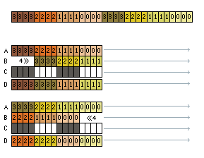
We have a 4 bit value per pixel, but a word has 16 bits to store them in. We can take advantage of this to duplicate the bits, placing them where we need them for the conversion. We repeat each bit x4: 3210 → 3333222211110000 e.g. 1010 becomes 1111000011110000. The source texture can be stored in this format, or converted in precalc using a lookup table.

Now the first thing we want to do is get rid of this duplication, combining four pixels into a single word, with like bits grouped together. We do this with two masked merges, combining odd and even words, and halving the buffer size on each pass. This is good news for the size of the remaining blits!
Ok let’s try to visualise the operation:
- Numbers represent bit indices
- Colour represents source pixel
- Arrows represent modulo, skipping words
- Letters are blitter channels
- Channel C uses static data as a mask. The minterm for this is
(A&C)|(B&~C).
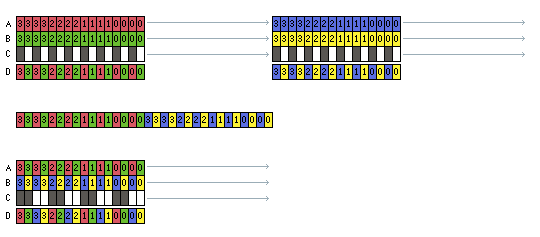
Now we have four pixels per word. This could also be our starting point in effects that can combine pixels as they draw by ORing values together. But what we really want is full words only containing the same bit number. We can do this using swap operations, first swapping groups of 4 bits, and then groups of 8. We can combine the second swap with copying the data to the destination planar screen’s bitplanes.
A swap consists of shifting and masking alternate words, to align the common bits. First shifting right (a standard blitter shift), and then left, which requires a reverse blit.
(Now we switch to using colour to show grouped bits to make things clearer)
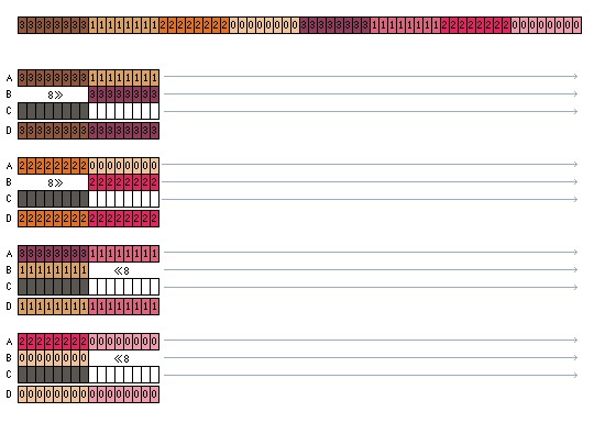
Now we’re done, and we have the image in separate bitplanes. In reality each of these passes will require multiple blit operations as the max blit height on OCS is 1024. I chain all the blit operations using interrupts, storing a count of remaining words, and a pointer to the next operation. I use this to chain it with other blit operations like clearing the buffer.
Soundtrack #
Now I’ll hand over to H0ffman to talk about the soundtrack…
The premise #
First let’s cover the top level. Gigabates is making an Amiga 500 demo, classic stock 512/512, very narrative and aesthetically driven, essentially pulling out all the stops. As is usually the case when making a demo, you’re not actually trying to beat the competition. Instead you’re trying to beat yourself (gigabates - I’d still like to try and beat them!). I get the feeling from our first discussions that he really wants to push this one so I guess we need to make sure the music is not only fitting the theme but also trying to push the limits a bit.
What does that mean? Well of course ProTracker will be the tool of choice, the reasons may be obvious to most of you reading this, but let’s just back track for the uninitiated.
ProTracker is a piece of music software for the Amiga which allows you to sequence music using a set of samples, 31 samples to be precise. It really is the de facto standard for composition on the platform and let’s be honest, it’s not good. It was built in the 90s, has terrible code and pointless restrictions. Despite all of its problems it quickly became the industry standard as it’s quite fun to use and has a lot of super optimised replay options.
The kicker is that sample data, even 8-bit, gets large very quickly and there’s only a finite amount of RAM and disk space available which all has to be shared with the demo. A standard approach is to give your musician a sample RAM budget. Stay in your lane and there will be no trouble. The thing is, I don’t like staying in my lane.
With a tool selected we pick our aforementioned replay solution which is LightSpeedPlayer. We’ll also need to consider how we’re going to try and push the technical side to get what we ( and I ) want. This will require some memory management and compression which all plays nicely with the demos’ multiple spinning plates. But hey, let’s not get bogged down with the technical just yet, we haven’t even placed a single note yet!
The emotional #
Gigabates spends some time with me explaining the premise of the narrative and demoing the work in progress code he already has up and running. A kind of nature vs technology story. At this stage of the process what you need are some reference tracks, a playlist of existing tunes which loosely fit the aesthetic. I’ve come into the project at a point where it’s pretty well realised and as such, Gigabates hands me a literal palette of music to listen to. Everything is centered around ambient / liquid Drum and Bass, be it modern tunes or classic era cuts from the 90s.
I’ll be honest here and say I probably listened to about five or so tunes. Most of the playlist is already in my music collection, so this is definitely my wheel house. The good thing about choosing this style of music is it has an organic and natural feel. The textures will come from real drummers, bass players, pianos, etc. Melodically there is usually some real emotional heft behind it. Soaring ethereal chord progressions and intricate rolling drum lines, yes please! Let’s imagine for a moment this demo having a chugging techno soundtrack…. Nope, it just wouldn’t work.
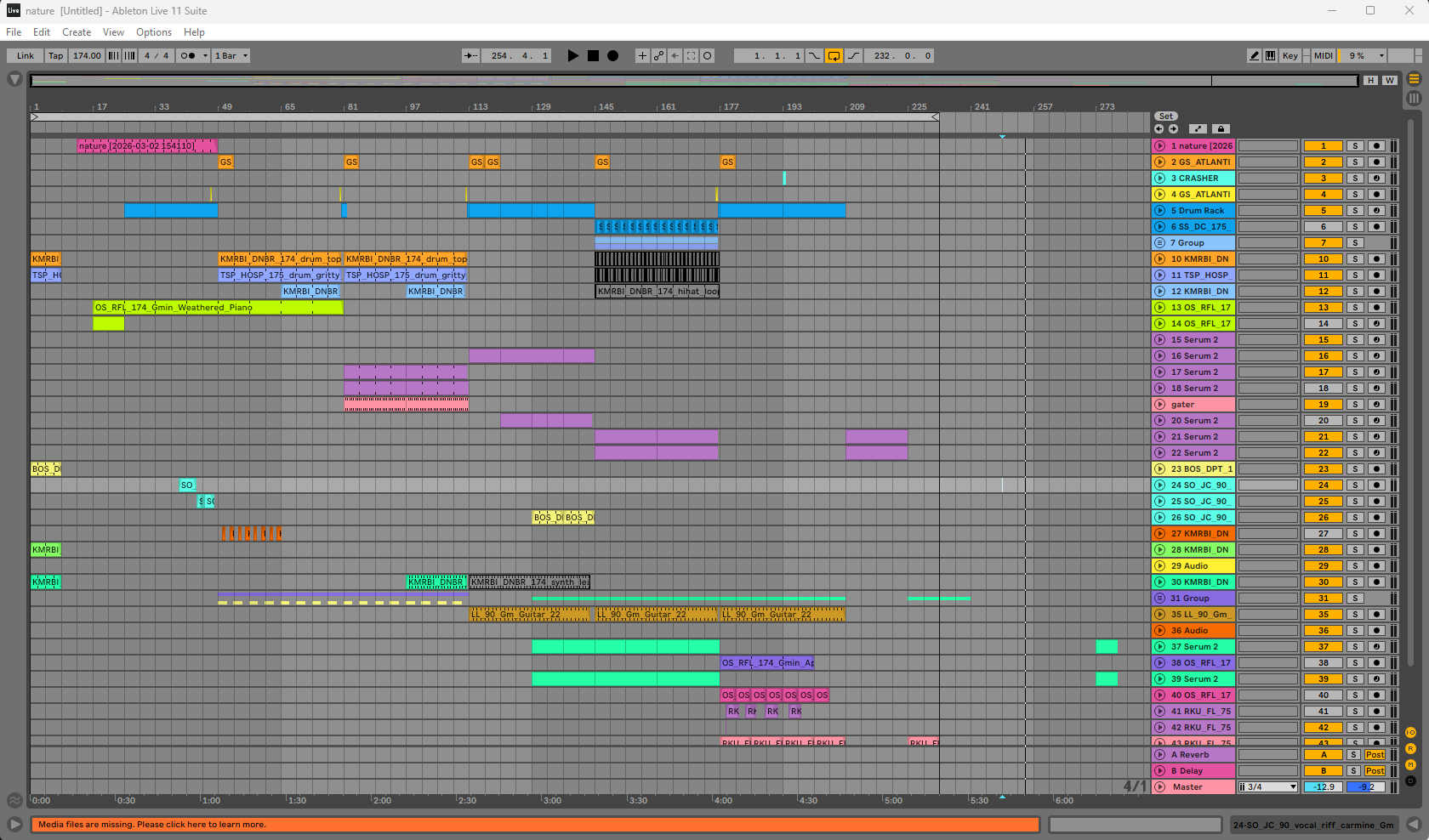
It’s time to start sketching out some ideas. As with almost all of my Amiga music projects, the process starts in Ableton ( other DAWs are available ). The key here is I have a work flow which is quick to jam with. I can spend a couple hours tinkering with some sounds and have something rolling very quickly. If it doesn’t work, don’t worry, you just throw it away and try again.
The demo storyline runs in three chapters, nature, technology then back to nature. For the first chapter I decided to use more natural sound, fretless bass, piano, strings etc. as these instruments are created from natural materials. The middle section will be technology so at that point I’ll need to layer in more synthetic sounds, arpeggios, reese bass and so on.
I spent an evening doing the first sketch. Kick things off with some bird song to really settle in the mood. I layer in a wistful piano line and some double bass. Lastly, some rolling drums on the softer side of Drum and Bass and we have our first sketch. As luck would have it our director and chief, gigabates, signs it off.
I continue to flesh out the music in Ableton, all the while keeping in mind that at some point this will need to fit in just four channels, not the thirty or so I’ve already managed to amass. How does that work? Just experience. Once you’ve done this enough times you end up with a bag of tricks and a forward thinking instinct on how to use them.
At any rate, we have a direction of travel locked in and about half of the music laid out in our DAW. It’s time to start getting this onto our intended platform.
The technical #
When making tracker music for a compo at a party, the file size limit usually rolls in at 2mb, which is very large. You don’t have to worry about size so much and can ramp up the sound quality. Within the confines of an A500 demo, that is not the case. Very early on gigabates and I agree on a budget, 200kb of chip (sample) RAM and around 50kb slow (data) RAM. This means the demo work can continue with that memory set aside before any music is available. It also gives me a “negotiable” guard rail. We also agree on 200KB of disk space, so some sample packing will be needed.
The process now is to export chunks of audio from Ableton as full 16-bit wav files, say a piano, some drums, and resequencing into ProTracker. However, the Amiga can’t just use that as is, it’s only capable of playing mono 8-bit samples and tops out around 28KHz. This means each sample will need to be re-sampled and have its bit-depth reduced.
It may seem obvious but resampling and bit reduction is a one way street. Once converted you want to avoid performing any further modifications to the sample as the detail required is now lost. So pro tip kids, keep your high quality source samples safe in case you change your mind. Another thing to note is the Amiga has 64 volume levels available on each channel. Why is that important? Well it means when you play an 8-bit sample at a lower volume it retains sound quality. At max volume, you can’t turn it up without changing the sample, but you can turn it down. This is why it’s important to make your 16-bit sources as loud as possible before conversion.
So the steps look like..
- Export from Ableton
- Make it mono
- Make it as LOUD as possible
- Resample and convert to 8-bit
At step 3 you could also add some additional processing, like EQ for example if you spot something which might need cleaning up or boosting.
Step 4 is where we need to be flexible. While the Amiga can play up to 28KHz, we can’t just have all our samples at that rate. I’ll run out of RAM very quickly but also I won’t be able to flexibly play instruments at different rates. I need a flexible resampler, thankfully I solved this a long time ago by making a little tool called Wav2Amiga.
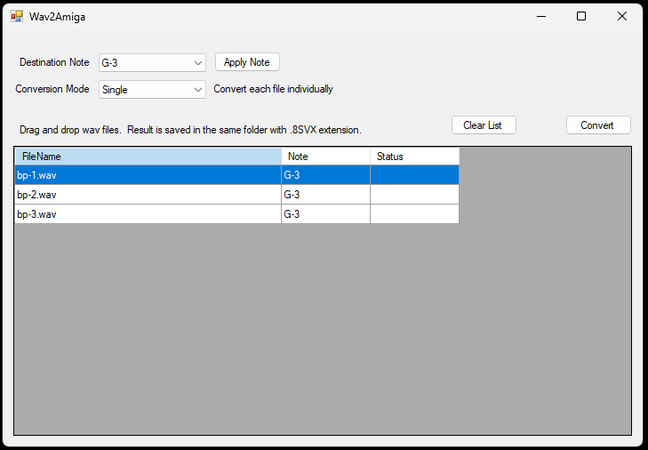
It’s very simple: select a destination note in ProTracker, drag and drop your 16-bit wav files onto the window and hit the button. It then resamples and converts them all to 8-bit and saves them with a .8SVX file extension in the sample folder. It also warns you if something you’ve converted is over 64KB in size, another little size restriction in ProTracker you need to be aware of.
The benefit here is I can exercise a little Nyquist theory, well with my ears anyway. The basic idea is your sample will have high and low frequency content. High frequency content requires a higher sample rate. So if your sample doesn’t have a lot of it, say a soft piano or a bass, then you can get away with reducing the sample rate.
You could break out a calculator at this point and do some frequency checks on your source but really it’s much quicker to just do it. Wav2Amiga allows me to quickly convert a sample at different rates. Load it up in ProTracker and take a listen, rinse and repeat till you’ve found the balance between result and size.
Sustaining Loops #
Now we’re onto a trick I never really thought to do until this project but it’s one I’ll be carrying forward for sure. First let’s look at the main piano line from Ableton.
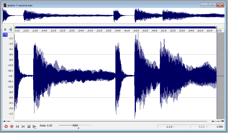
There’s five chords here with some pretty long tails, that’s gonna be very expensive. On closer ear inspection you’ll notice two of the chords are incredibly similar so we can afford to lose that detail and get ourselves down to three samples right off the bat.
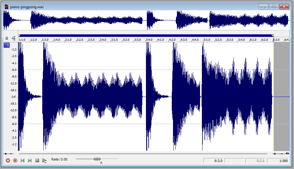
What to do about those long tails though, we need these things as small as possible? Well you can set a sustaining loop in ProTracker and use the volume to gently fade it out. Sadly due to the hardware, this loop is only in one direction. If your sample has some kind of phasing or decay in it, you end up with an almost percussive jolt each time it loops round.
To solve this I drop the samples into the sampler. The two chords with the long tails I setup a ping pong loop with some cross fading. As you can see we’ve effectively thrown away a lot of that sample.
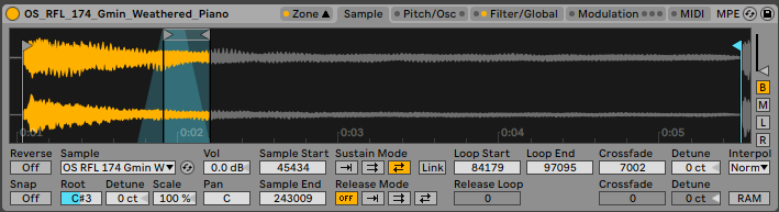
With that all in place, I can export each of the samples with the ping pong loop applied continuously. When that arrives in ProTracker, I’ll have a much easier time of creating the loop. Admittedly you do end up with a kind of rotary / circular effect, but this is far better than jolting or clicking.
Bonus Tip #
Another similar technique is for short samples with long reverb tails. If your reverb has a freeze function, add automation to switch on one after your sound has played. The reverb tail then stays at a constant volume, making it much easier to apply a ProTracker sustaining loop on it.
Distant Memories #
The first half of the music is now in place in ProTracker and takes just over 200KB of sample RAM, so now it’s time to consider our options for what’s next. This isn’t my first time streaming samples to beat memory restrictions. My first experience was working on Eon with The Black Lotus. They had the demo system fully integrated with a sample loader and my loop mixer with a full timeline. More recently I made the Tactical Transmissions music disk which streamed samples and played a continuous techno DJ set for 45 minutes. For this project I’ll be repurposing some of the tools I built for the latter.
At the core of this is a memory allocation system. When you look at how a piece of music “generally” works, the instruments you use will come and go. For example, the large bird song sample in the intro plays for a number of patterns and doesn’t get used again. That vocal, only used for about eight patterns. So why leave these occupying memory when we could use that for new sounds later on?
The first step is knowing what is played and where. The tooling I have already had this simple output. It runs through the mod file and sees which sample numbers are used on which song positions. It’s not super clever, for example fading a long sample out over a few patterns will trip it up if the sample number isn’t there.
We can now determine when a sample needs to be loaded and when we can re-use that memory.
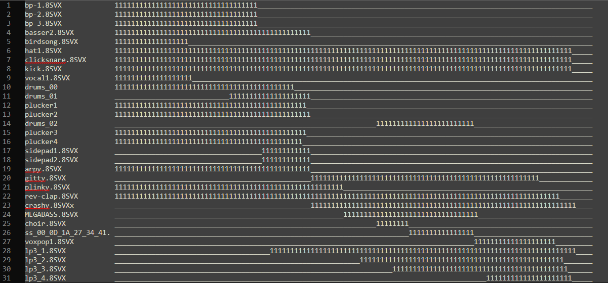
Sample names down the left, song positions across the top
We know what is required and when. Now we need to formulate a plan of where. Now you could build a memory allocation system which runs in real time on a 68000 but that will get messy and really it’s just a waste of cycles. Instead I pile the start and end points into a memory allocation program in C#. This steps through each position allocating and deallocating samples. The end result is effectively a sample ID and where we need to load it in the buffer.
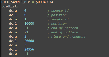
Tactical Transmission Loading List
Integration #
Now we need to work out how we load these samples. There is an already bustling demo system which is loading demo parts from the disk and abusing interrupts left right and center. I chat with gigabates about potential approaches, how we might interleave the sample loading with the part loading but it seems like we might need a slightly less intrusive approach.
He suggests that instead of loading each sample individually, we pre-load the 200KB buffer with everything that is needed from the start. Like a mod missing half its samples. Well, that really does simplify things to get us up and running but what about the runtime stuff later on? How about we pre-load those as well? This is where the compression comes in.
All samples are packed with the 4-bit delta compression as used in The Player 6.1 many years ago. It’s a lossy method but it halves the sample data and allows us to compress it further when putting it on disk. But the real benefit is the unpacker uses a simple look-up and a few instructions. Super lean. I’ve spent way too much time with this encoding, so I already have the most optimised method of unpacking.
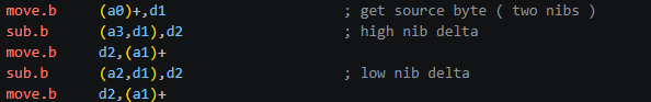
Optimised 4-bit delta unpacker using two 256 byte look-up tables for speed
We could potentially plug the sample unpacking into the demos loading system but it seems like a lot of complexity to interleave these two things together. Instead I came up with a plan to use the existing music CIA interrupt. I know what the coders are thinking right now, “What are you doing man, unpacking data in a high priority interrupt?! That’ll kill everything”. But, if you only unpack a tiny bit at a time then the impact is minimal. I modify the tooling to produce a plan of what needs doing based on the music frame.
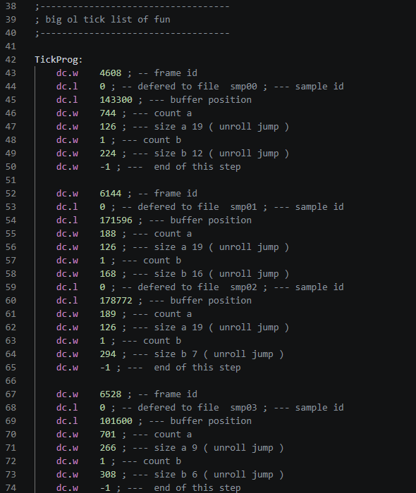
The tooling sees it needs to load a set of samples four patterns before they are played by the music. It totals the number of bytes it needs to process and distributes that across the number of music ticks. It also handles all that messy business of there being a remainder number of bytes left to do. Before I get too deep in writing the 68000 side, I need to check what our maximum byte per music tick will be which rolls in at 23 bytes.
I set about building the player / unpacker which will also serve as my testing rig for the soundtrack. You’ll see in the video the two raster colors, Red is the LSP replay and Blue is the sample unpacking.
Taking a rough estimate and comparing it against the stats on the LSP page. Even with the unpacking and player code combined, this method is still faster than The Player 6.1 on its own. Well, that depends though doesn’t it? This is now music data dependent, so if I trigger 150KB of samples in one place the number of bytes per tick will increase. We need to be careful about this and in fact we might need to see a little more detail on what’s going on. For now though, we plug in the new runtime sample unpacker into the demo system without any trouble and we’re off.
The Manual Touch #
The tool belt is now full and everything is up and running, which leaves us with the task of finishing the music. By now most of the demo parts and layout are in place so I get to work fleshing out the remainder of the soundtrack. This is mostly an iterative process, laying down new parts, checking gigabates is happy with the direction and mood, putting stuff in ProTracker, all while keeping a check on disk space and memory.
Everything seems to be rolling in with no issue and no clashes, except at one point the rotozoomer effect starts to drop frames. I fire up the soundtrack tester and see that around that section the unpack is doing a lot of work. I think we might need one more tool. I need to see what the memory looks like at each song position, so I draw up an HTML output displaying all the steps.
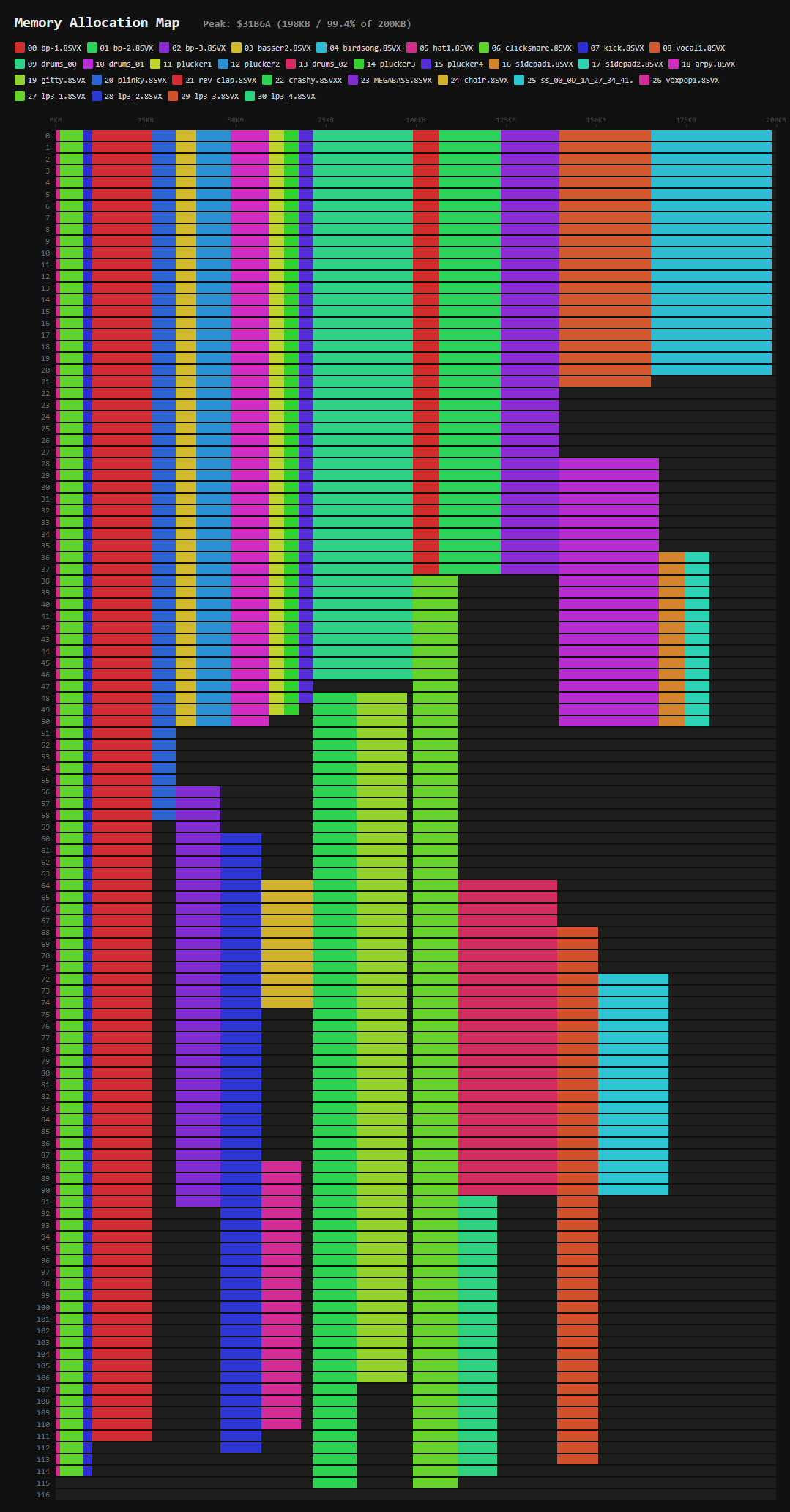
Note: this is the final altered memory map
Using this I can now see how much free RAM is available at every point. Now I can do a little cheating. Looking at the map I can see there is plenty of RAM available well before that part is active, so I add a silent trigger for samples used later on. This is something you can’t hear, but it tricks the memory allocator to load the sample much earlier than it needs to. The result is it distributes the sample unpack across a larger space, reducing the hit on the frame time.
Wrap-it Up #
The tune gets finished and the final parts of the demo are coming in gradually as Revision approaches. We locked down the soundtrack at this point so we have a known quantity we can work around. At this point (four days before Revision) it’s looking like it’s a done deal.
Part breakdown #
Next I’ll go into the implementation of each of the demo parts.
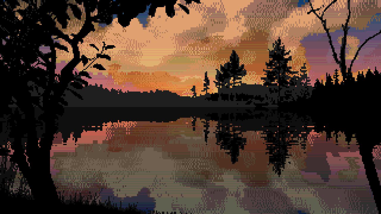
Title screen #
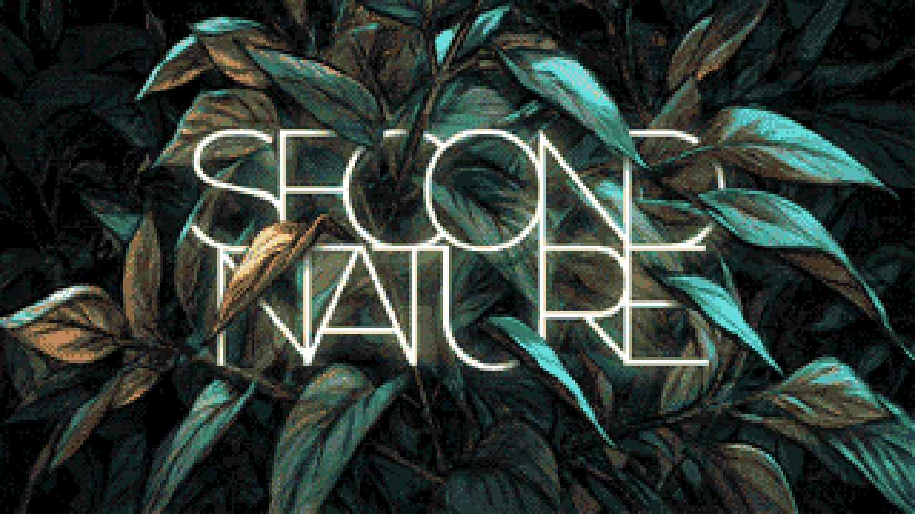
We start with an image based effect to set the mood. Steffest created this great logo screen, and when I confirmed we had enough disk space (which was true at the time!), he extended it so we could pan up into the sky as a transition to the next part.
To suggest some neon light flicker, I added a palette transition linked to a random noise table. There’s a gradient on the sky that scrolls at a different speed to the image, giving a parallax effect. The gradient was created using my Gradient Blaster tool.
Leaves #

This is the part everyone seems to want to know about! Contrary to what some people have suggested, it does use realtime texture mapping. It just uses some smoke and mirrors to reduce the amount of work needed.

the leaf texture
The main trick is that there are actually only two leaves. On every frame we draw one big leaf and one small one, with a two bitplane c2p mode, and a texture mapper routine similar to the one I’ve used before. These are drawn into a 16 frame cyclical buffer, and each of the visible leaves is blitted from a different frame offset in this buffer. This gives the appearance of different leaves, where in fact they’re just the same leaf at different points in time.
Each leaf instance is blitted into our main planar screen once the blitter is done with the c2p. The screen is 5 bitplanes, and the big and small leaves are written to separate bitplane pairs. The credits text is drawn to the remaining plane. These bobs have enough white space padding, and move slowly enough that they are self-clearing and don’t require any restore. The blank pixels around the leaf are enough to wipe out the previous frame.
The leaves are carefully positioned to not overlap vertically within the same group, so that each instance can have its own palette via copper splits. These are dynamically inserted between the leaves. The palette is selected based on the angle of the leaf, so we need to store the angle of each of the 16 frames in our buffer. This gives an approximation of flat shading, and I think it does a good job of hiding the low bitplane count of the texture.
Copper splits setting the palette for each leaf
For the movement of the leaves, I use a Perlin noise table to give the appearance of random movement, with a constant applied so that all leaves drift in a common direction. I also add some variance in the Y position so that the leaves are not exactly evenly spaced, but still ensuring they don’t overlap.
I use bitplane palette tricks to give the appearance of transparency on the text. Basically for the small leaves I generate a lighter version of the palette where they intersect with the text bitplane. This is generated at runtime, as the text needs to fade. The sun burst in the background is made of sprites, with priority set to appear below the bitplanes.
Ripples #
This is the first effect I coded for this demo. The main code was written while waiting in the airport coming back from 68kInside last year!
It’s similar to the radio waves effect at the end of Desire FM. Here I had concentric rings radiating out from the center of the screen, which formed a mask where the image was offset by a few pixels. In this version I plotted and filled the circles in realtime on each frame, which put a hard limit on the number of rings.
The idea for the new version was that I could have as many rings as I want, using the ‘infinite BOBs’ technique. Again this uses a cyclical buffer, looping over 16 frames. It only draws the outermost ring, overdrawing previous frames as it loops creating an infinitely expanding, repeating pattern. Well, at least until the radius reaches the dimensions of the buffer! To speed things up further, I precalc the x positions per line for each radius, and take advantage of symmetry. I only need one half of the mask vertically, as it can be applied in reverse with negative modulo for the bottom half of the image.
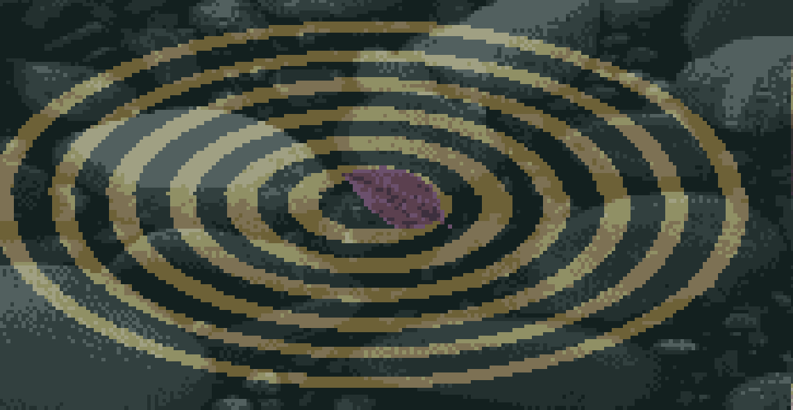
The area inside the mask is shifted by the blitter. The shift amount decays as the rings expand, to eventually disappear, before the next leaf drops and the cycle starts again.
To present the effect, I use prerendered sprites for the leaves, which are synced to the music. The screen setup uses five bitplanes, with three for the water surface, and two for the river bed. These are scrolled at different speeds for a parallax effect, and use more palette tricks for pseudo transparency. The mask effect is only applied to the surface bitplanes.
The merged palettes are generated offline in JavaScript, using the ‘soft light’ blend mode, that you might be familiar with from Photoshop. Figuring out the palette order for this takes a bit of thinking about. The reflection layer uses bits 0, 2 and 4, and the riverbed layer uses bits 1 and 3. This gives the colour indices 0, 1, 4, 5, 16, 17, 20, 21 and 0, 2, 8, 10 for the two images (see the binary lookup table below). All remaining colour indices are sums of the colours which must be blended. e.g. color03 would be a blend of color01 + color02.
pf1 bpls 0,2,4
0  1  0  1  0  1  0  1 (1)
0  0  1  1  0  0  1  1 (4)
0  0  0  0  1  1  1  1 (16)
0  1  4  5  16 17 20 21

pf2 bpls 1,3
0  1  0  1 (2)
0  0  1  1 (8)
0  2  8  10
Clouds #
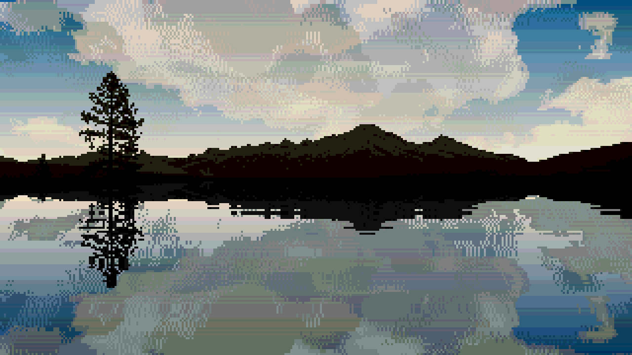
Time lapse footage of clouds seems to be a common trope on liquid drum and bass videos. In common with the music, there’s a contrast of high speed with relaxing vibes which I really like.
This effect uses bplcon1 scaling to achieve a perspective effect on the clouds. This is a technique that allows us to skip up to one pixel per 16px word by adjusting the scroll register with the copper, essentially giving us hardware scaling to reduce the width of an image by 1/16th for free. This works because if you decrease the scroll amount mid-line, the last pixel in the current word is not drawn, and the next word starts early. To scale beyond this threshold, I combine it with 5 prescaled versions of the cloud image. For the vertical scaling part of the perspective effect, we simply skip rows using bitplane modulo. The scaling is simply applied in reverse with negative modulos for the bottom half, with the addition of a water ripple effect, which we’ll get to shortly.
Replacing the clouds with vertical stripes to visualise the horizontal scaling
The clouds consist of three bitplanes: a two bitplane image and a single bitplane image interleaved into one. The two images are vertically scrolled independently at different speeds by setting the bitplane pointers, giving a parallax effect, and use another palette based transparency effect. The cloud image tiles vertically and repeats so we can have a continuous loop. The remaining two bitplanes are used for the tree/mountain horizon overlay. These are unaffected by the scroll offset scaling and perspective modulo, as these are set independently for odd and even bitplanes.
It would have been nice to add a sun / moon using sprites, but this is prevented by a couple of factors. Firstly because we use all 5 bitplanes, we don’t have a separate sprite palette, and the lightest colours aren’t where we’d need them. Secondly, the sky doesn’t actually use the transparent color00, in order to keep the overscan borders black.
The water ripple effect uses an animated sine wave to offset the line Y using modulo. This is a pretty classic OCS effect, but a few things make it a bit more fiddly. It needed to incorporate the perspective effect so the waves get smaller towards the horizon. This isn’t too hard though. We just precalculate a table offset per line, and then animate the initial offset into the sin table. What was a bit of a pain is that for the cloud bitplanes we’re already using the modulo for the perspective scaling. I solved this using generated code to add the base modulo per line to the sin result.
The next part of this effect is the animated gradients. These are calculated in realtime, setting 8 colours per line across 160 lines, giving a total of 1280 RGB colours to calculate and write. This required some significant optimisation!
My solution was to store the RGB values in fixed point, spread across a longword and two words, with the bits placed exactly where we want them to recombine into a single RGB word without shifting.
gggg_Rrr
    bbGg
    ___B

uppercase = integer part
lowercase = fractional part
_ = unused
I use this format for the current RGB value, and the delta to be added on each step. Incrementing each step is simply three add operations at just 16 cycles. addx carries up to the next component.
        add.l   a2,d0 ; gggg_Rrr
        addx.w  d3,d1 ;     bbGg
        addx.w  d5,d2 ;     ___B
Combining these back into a single RGB value just requires masking and adding the components together, and is also just 16 cycles.
        move.w  d0,d6 ; _Rrr
        move.b  d1,d6 ; _RGg
        and.b   d7,d6 ; _RG_  (&fff0)
        or.b    d2,d6 ; _RGB
To achieve the dithering effect and avoid harsh colour bands, I use separate deltas for odd and even lines. One adds an extra fractional amount in order to round up, and the other subtracts this again.
As well as interpolating the gradients within a single frame, we also want to animate the palette over time to simulate the transition from day to night. This means also interpolating the start and stop values for each gradient, as well as the fixed colours for the horizon. I store a fixed palette for every 128 frame interval, and then interpolate between these in a similar way. To generate these palettes, I created each screen in Photopea (a Photoshop clone) in true colour, using layer effects, transparency etc to get the desired result, and then used a script to sample the RGB values at specific pixel coordinates to build the palette.
Overall what maybe looks like a quite a simple scene ended up being a copper list from hell and leaves barely any raster time left, barely giving us time to load the next scene!
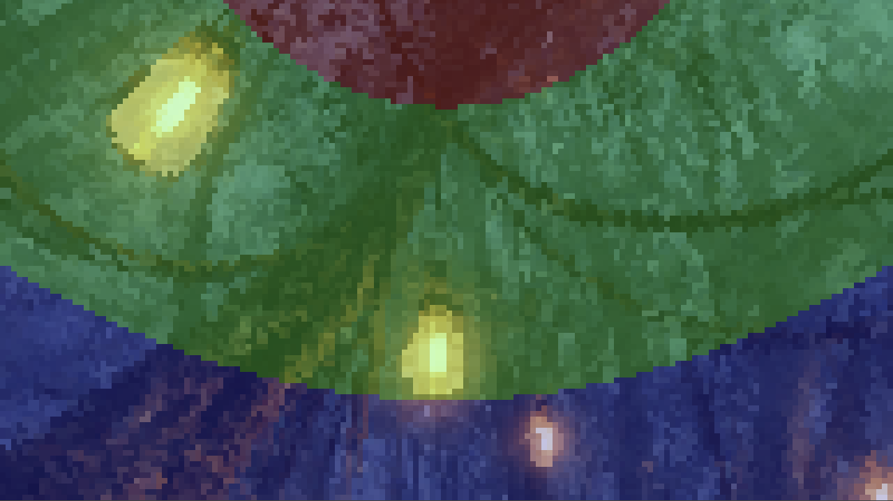
Tube Lights #
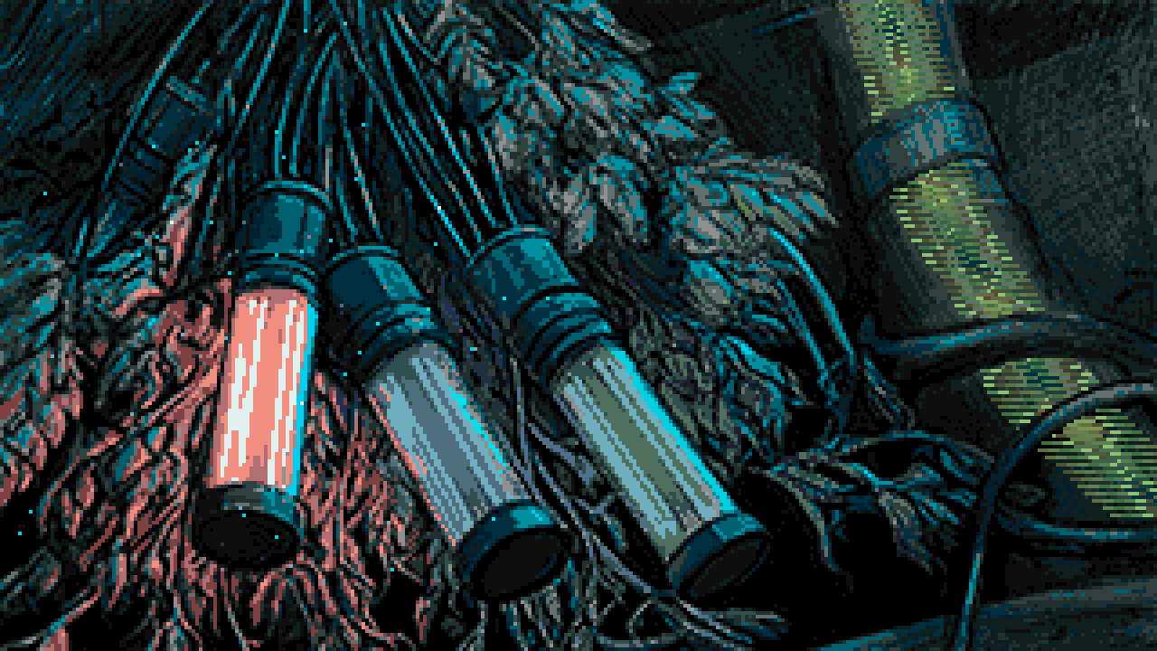
This is the first of Steffest’s awesome palette trickery based effects. Having been blown away by his incredible AGA colour cycling piece The Vision, I was excited to see what we could do in this demo using palette effects.
The way this works is by dividing the palette into a separate range per light source. When the lights are off, the colour values for these ranges are the same as the base palette, requiring some duplication. When we fade one of these ranges to the ‘light on’ palette, only the pixels lit by that light source are affected.
To complicate matters slightly, the yellow tube on the right hand side shares the palette range with the leftmost light. This required a horizontal copper split, waiting for the x position just after the light, and setting the animated yellow palette on each line.
The icing on the cake was adding the fireflies ‘particle’ effect over the image, and making them attracted to the active light source. I’ll cover the implementation of this in a later part, where we use the same logic for a much bigger version.
2D Tunnel #
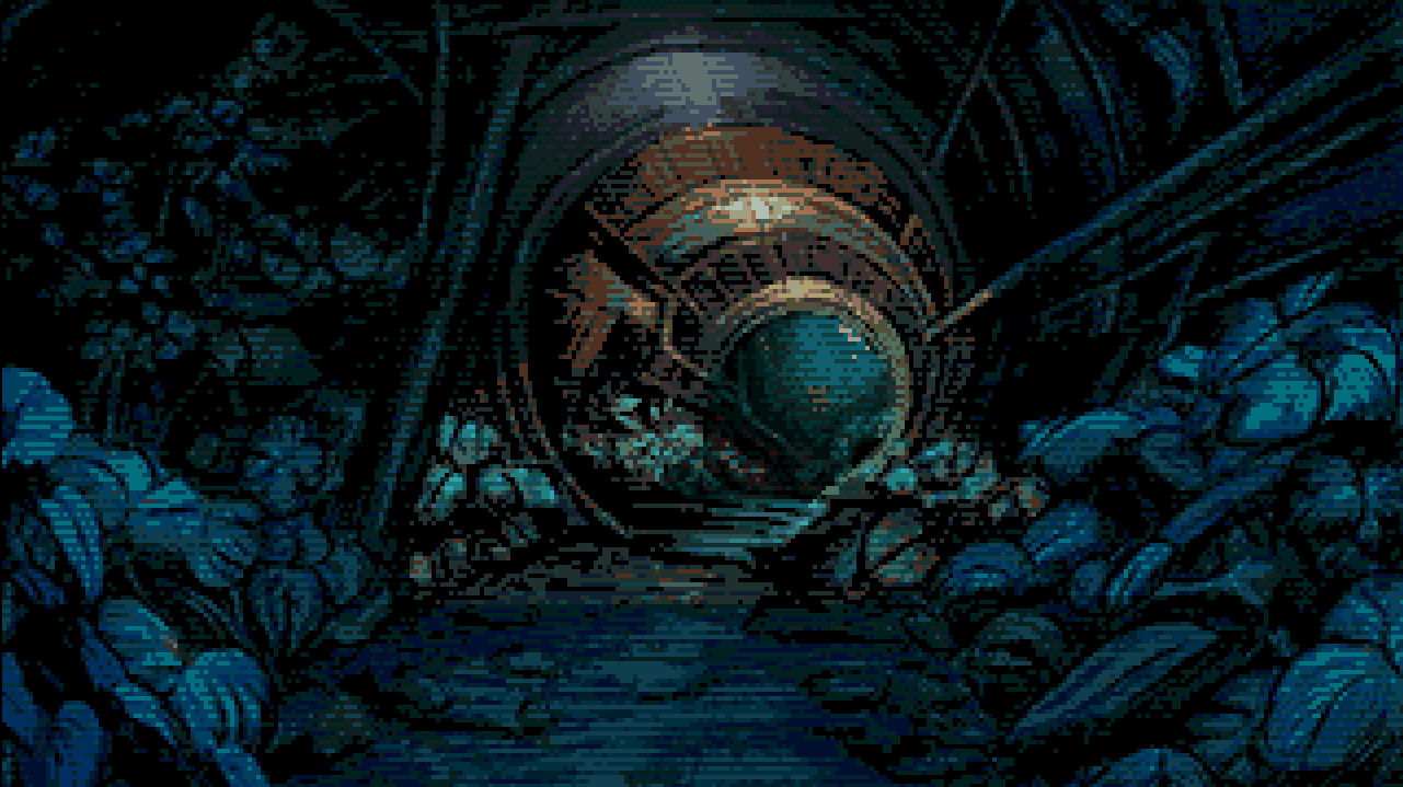
This is another palette fading part, similar to the previous part, with another incredible image from Steffest. This time it uses Extra Half-Bright mode to take advantage of a full 64 colours.
Chunky Tunnel #
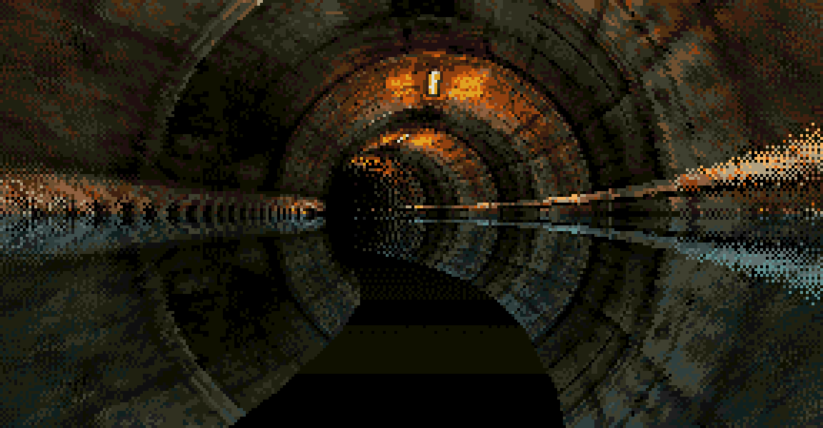
Next we transition into a technical effect, with a pseudo 3D version of the tunnel we just saw. This is a table effect, using my new 1x1 4 bitplane C2P routine, which I detail elsewhere in the article.
The geometry for the table was created in Blender, using a gradient texture to output the UV offsets as RGB. The scene is just a camera inside a giant torus, with a plane intersecting to provide the floor.
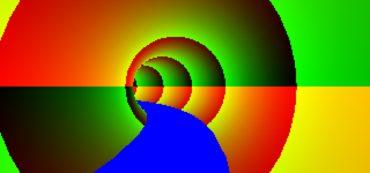
UV data exported as RGB from Blender
Data is then extracted from the rendered image to generate the table data used by the Amiga program. One additional step that happens at the conversion stage is the addition of dithering to add a fake depth of field effect. For the pixels closest to the edges, where the large texels would be most visible, this is smoothed by applying a Bayer pattern, shuffling the pixels to simulate blur.
Eventually the UV offsets need to be transformed into huge unrolled series of move and or instructions. While we could just generate the instruction code offline, this doesn’t compress very well. Instead the offsets are exported as delta tables, separated into U and V. The init code on the Amiga then transforms these into the code.
While the chunky to planar process is actually pretty fast, the real bottleneck is just drawing the pixels in the chunky buffer with the CPU. We just don’t have the capacity to fill a full screen buffer at 1x1 resolution at any reasonable frame rate. The optimisations have to be around avoiding drawing pixels. The big trick is that we only draw the top half of the screen and mirror it using negative modulo. The obvious giveaway would be the lights on the floor, so we cover them up with sprites in the shape of the floor plane! The bottom half also has a different palette, using cooler colours, and the orange glow removed.
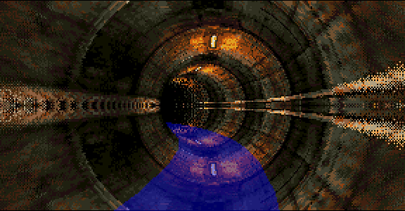
Sprite overlay hiding the mirroring
The solid sprite as a floor is a bit underwhelming, so I added some animated copper bars to give the impression of lighting from above.
Zoomer #
Probably the part that caused the most pain, and definitely the one that burnt the most disk space!
This is an incremental bitmap scaler that works by inserting columns using the blitter to achieve the horizontal scaling. Vertical scaling can be done for free using the copper of course. I’d previously implemented a simple scaler using this method, and never used it for anything, but I’d always had in the back of my mind how it could be used for an “infinite zoomer”.
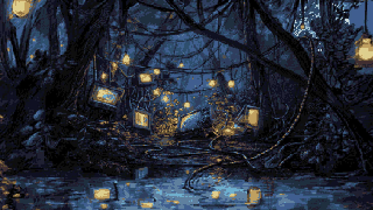
Steffest created the original high res image 2560x1440, which was split into three zoom “levels”, plus an additional foreground layer on the first level.
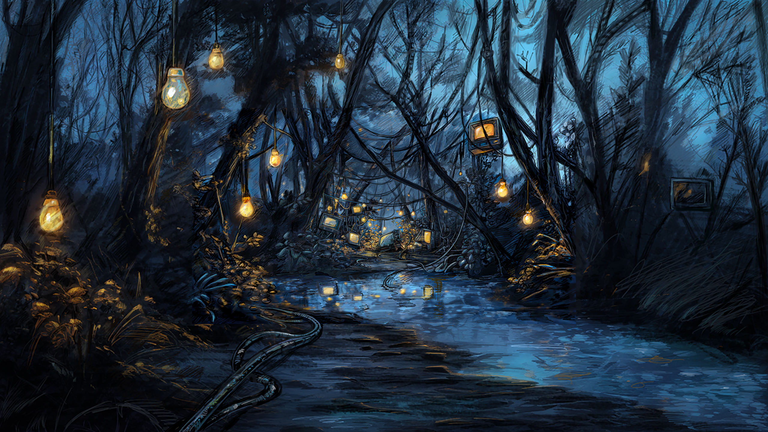
Original high res image
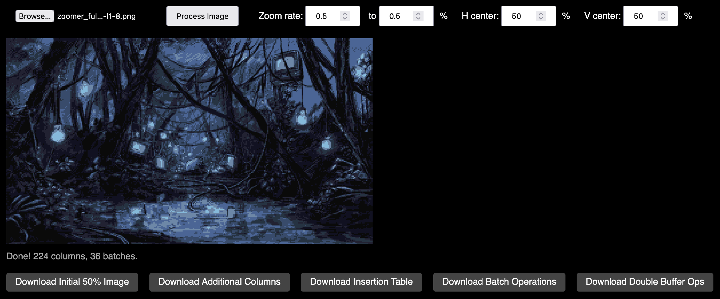
For each layer we start off with an initial image state at 50% width (320x360) i.e. only containing the even columns, and another buffer containing the additional columns which are not yet displayed. We don’t quite need all the odd columns, because some of them would never be displayed, due to being off-screen by the time they’re “visible”. One by one the additional columns are inserted into the image. To do this we shift part of the image off the edge of the screen (either left or right) to make a 1px gap, and then blit the missing column into this space.
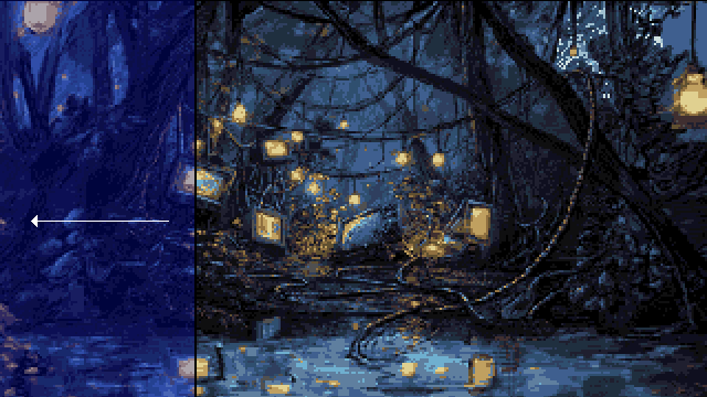
Shifting to make space for column insertion
This is repeated until all the additional columns are inserted and the image reaches 100% scale, at which point we swap the buffers to start at the beginning of the next zoom level. We don’t actually have memory to load all the levels upfront, so they need to be background loaded from disk. This is where some of the pain comes in, as it’s quite timing sensitive!
I built a JavaScript based tool to generate the data for the insertion operations to perform each frame, and export the image buffers. Calculating the order to insert the columns in order to give the appearance of natural scaling is somewhat challenging, because unlike regular nearest neighbour scaling, once a column is visible, it remains visible. The algorithm I used chooses the column at each step that introduces the least error, compared to the ideal floating point position of each column.
One annoyance is that because the screen is double buffered (and it needs to be so we don’t see the gaps mid-insert), we need to repeat each incremental step twice. The zoom speed is limited by how many columns we can insert per frame. The time taken to insert a column is quite variable, because the size of the block being shifted depends on the distance from the center of the screen. For this reason I allow the updates to fall behind schedule and then “catch up” again on subsequent frames.
The first level is actually dual playfield with two layers zooming at different speeds. The foreground tunnel layer is actually 2 bitplanes, but at the last minute we reduced it to only use one colour for disk space reasons. This also limits the palette of the main image to 8 colours, so we start off in monochrome with the lights off, only turning them on on the next level with a palette fade. There are actually several palette transitions during the zoom that make things feel a bit less static.
As well as the dual playfield part, we also have a static moon sprite peeking through the trees, to add to the perspective effect. This was partly inspired by this video about Disney’s multiplane animation technique.
https://youtu.be/YdHTlUGN1zw?t=159s
Fireflies
Once the zooming finishes on the final level we switch to a different effect: the full version of the fireflies we saw earlier. This is a particle effect which plots 1024 dots swarming around a point. As you might imagine, calculating and drawing this many dots would be very CPU intensive, and requires some optimisation techniques.
For each particle we have a coordinate pair, and a delta i.e. its velocity. On every frame we add each particle’s delta to its current position. As each component is a word, we can apply both X and Y delta into a single longword add. We don’t need to worry about overflow from Y into X.
      move.l  (a0)+,d0
      add.l   d0,(a0)+
Rather than looping over and plotting the particles, we’ll use the blitter to convert fixed point coordinates into bchg instructions, with one pass to generate the byte offset, and another to populate the bit index. This relies on the screen width being a power of 2, so we extend it to 512. This gives us a single unrolled chunk of code to plot the dots as fast as possible.
But why bchg and not bset? Rather than plotting the dots onto their own bitplane, we XOR them into bitplane 3 of the image. This flips colour indices from the upper and lower halves of the palette, giving some appearance of transparency. There’s another advantage of XOR though. Instead of clearing the dots, we just run the same generate draw code again, and the bchg instructions will flip the pixels back to their original value. Because the screen is double buffered, the draw code needs to be too.
The initial deltas are random, but to stop all the particles just zooming off the screen in a straight line, we need to periodically update these according to some algorithm. A key optimisation is that we don’t need to update all of them every frame. In this effect I update 1/8th of the particles, but this could really be much lower. The basic formula for the new delta value is:
- Damp the current velocity
- Add a new random value
- Subtract some fraction of its distance from the ‘attraction point’
The result of this should be that the particles swarm in a randomly changing direction, weighted towards a single point. We can change the location of this attraction point over time, like we did on the ‘tube lights’ part.
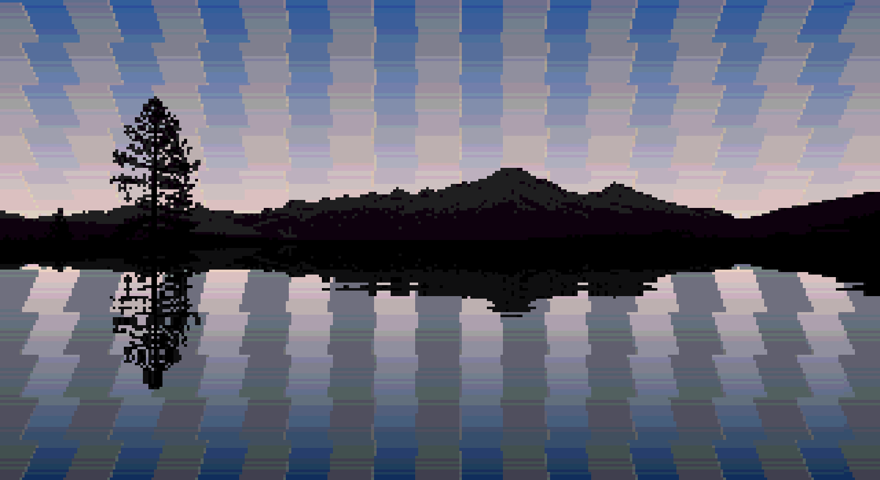
Tubes #

Another Steffest image / palette based effect. The plan was to have a few of these “simple” effects to use for preloading memory intensive effects that I can’t transition between directly.
As with all of the palette effects, Steffest provided a JavaScript based prototype, making my life much easier. https://box.stef.be/amiga/demo-toolbox/tubes/
When it came to actually implementing this, it turns out that having two groups of copper bars moving independently in opposite directions isn’t entirely “simple” after all! The solution was to build a data structure for all of the palette splits, and sort them by Y position using radix sort before writing them into the copper.
A bit of sync with the music leading up to the drop and it did the job exactly as intended.
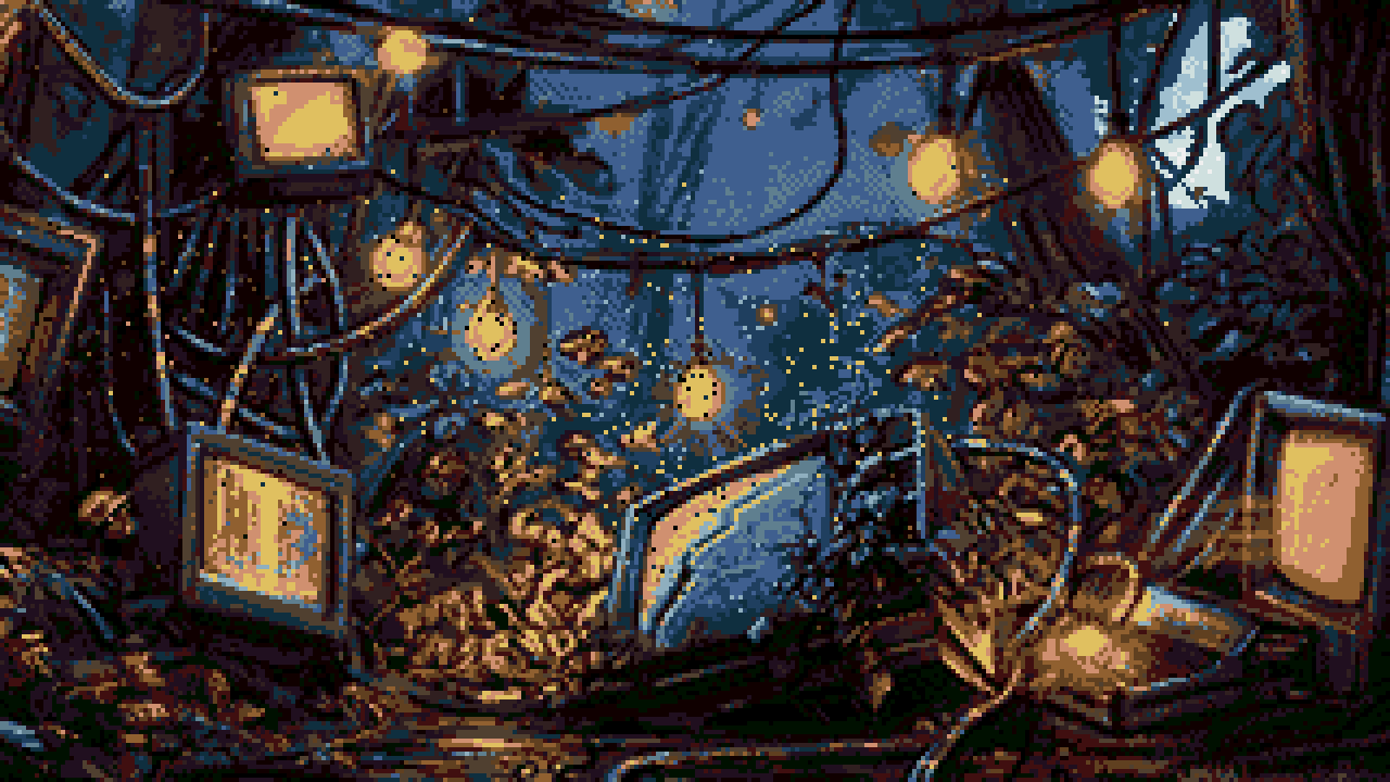
Sphere Map #
I’d always been impressed by the sky box effects on AGA demos, like The Martini Effect and other Flex productions, and notably TRSI/Mystic’s Lupus Reditus last year. As always, my mind goes to “how could this be done on OCS?”.
Initially I went down the route of cube projection, using my texture mapper routine. This would have been feasible, but probably not at a comparable screen size and frame rate. The more I looked into it, equirectangular sphere projection appeared to be an interesting alternative. While it definitely wouldn’t be possible to do a “correct” implementation in realtime, I kept coming back to the idea that it would be possible to do a simplified version as a table effect. And that’s exactly what I was able to do. Whereas on a real sphere projection the view angle varies per line as you’re looking up or down, in my simplified table version each line is drawn as it would be when centered in the viewport. This means that panning up and down the sphere is as simple as scrolling up and down the table. I’m sure I’m by no means the first person to figure this out, but it was fun to arrive at the solution independently!
All of this means that the hard part is the data generation, but once we have a table, it’s no different to a tunnel, or similar effect that I’ve done before. I render it using a 2x2 HAM7 chunky mode, similar to the one I used ( and tried to explain) on Bacon of Hope.
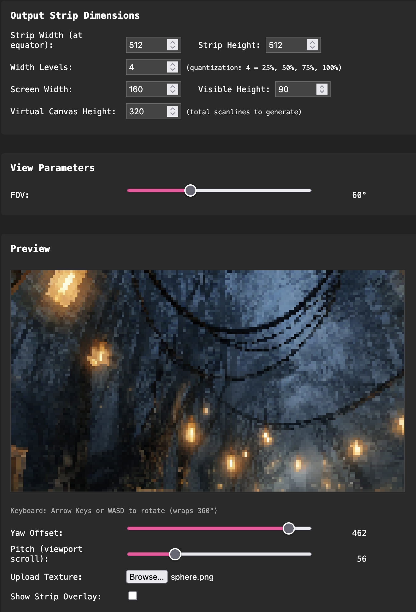
As usual I built a web based tool to preview and generate the data for this effect.
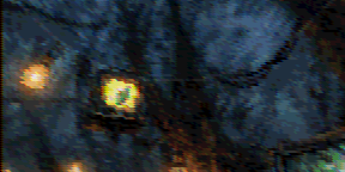
Another challenge was that the texture needed to be pretty huge in order to get non-blocky output. I realised that the equirectangular source texture was pretty wasteful, in that it contains way more detail than needed at the top and bottom due to the way it’s distorted. To take advantage of this, I split the texture into strips, scaling each one to the level of detail required. The limitations were that:
- images can only be up to 64k while being addressed from a single register
- we can only have as many strip images as free registers (5)
We can however merge strips of the same width where they fit within the 64k limit.
The data generation tool takes care of this splitting, and previews where the boundaries are:
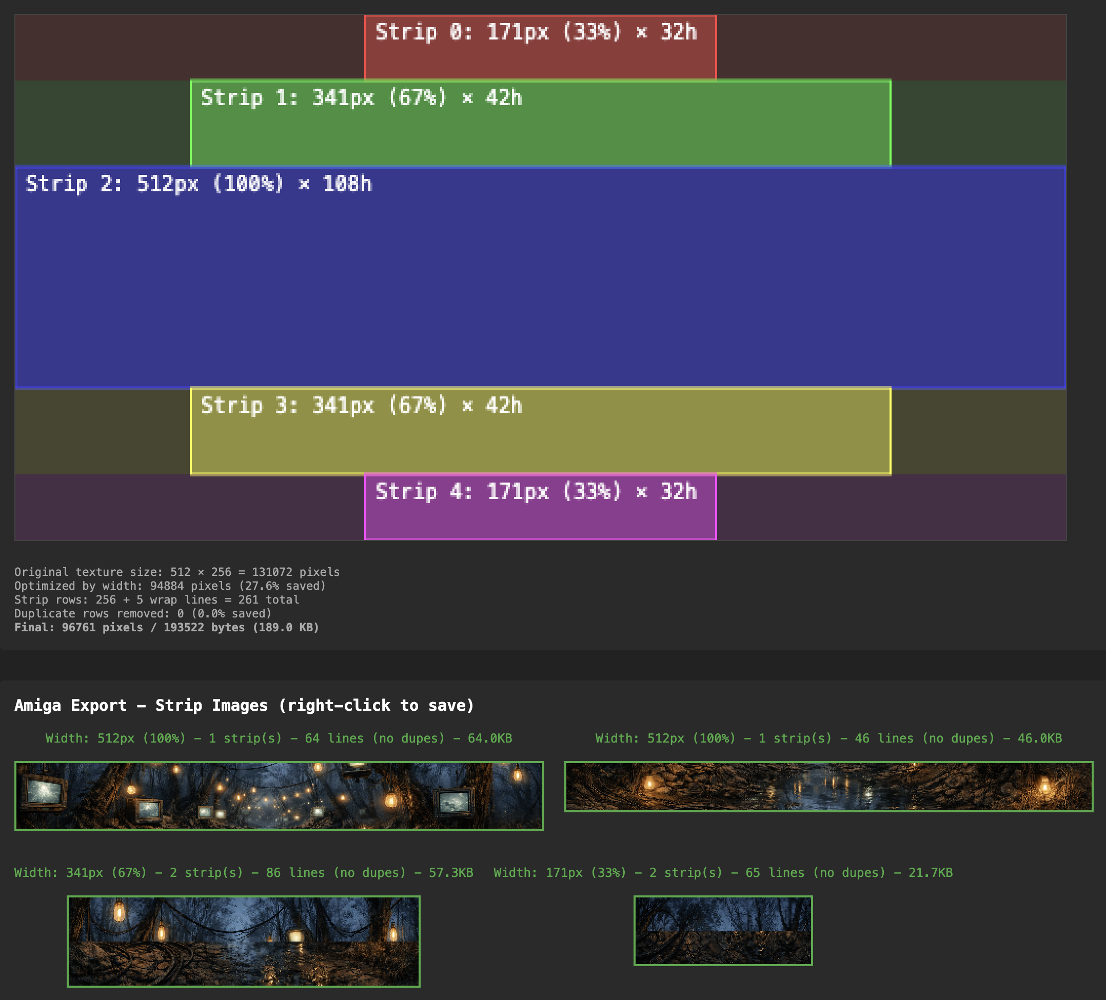
The movement animation is controlled using splines. I found that Catmull-Rom splines were pretty straightforward to implement on the Amiga side, and quite nice to author too, as it’s just a list of coordinates at key frames which are smoothly interpolated without the need for control points etc. Making this animate very quickly hides a multitude of sins, and fits nicely with the drop in the music. The eventual stopping point over one of the screens leads us into the next part…
Plasma #
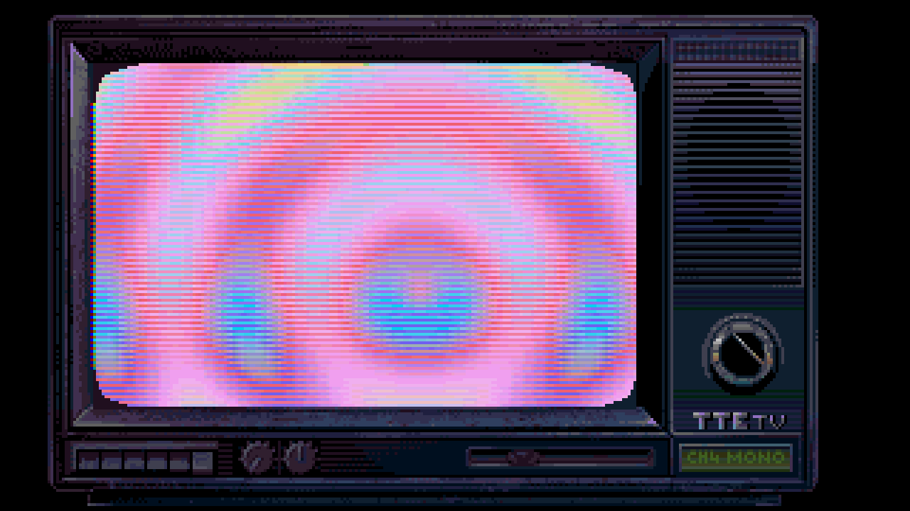
The next two parts are really just a creative way to insert a couple of more traditional demo effects into the narrative. I had the idea to use CRT bezels to add some framing to parts which couldn’t run in full screen. The left and right borders are sprites, and the top and bottom are just bitmaps with a copper split. All of this frames another HAM7 2x2 screen in the main area.
Instead of just doubling the pixel height with the copper, I tried to do something interesting with the alternate lines. The red and blue channels are swapped, and there’s a four frame delay on these lines. This gives a kind of motion blur effect where the colours separate as the lines diverge, and generally fits with the appearance of scanlines on the CRT.
For the plasma itself, it’s a pretty standard non-faked sum of sines implementation, with a radial sine wave added to a linear one to get the palette offset.
Rotozoomer #
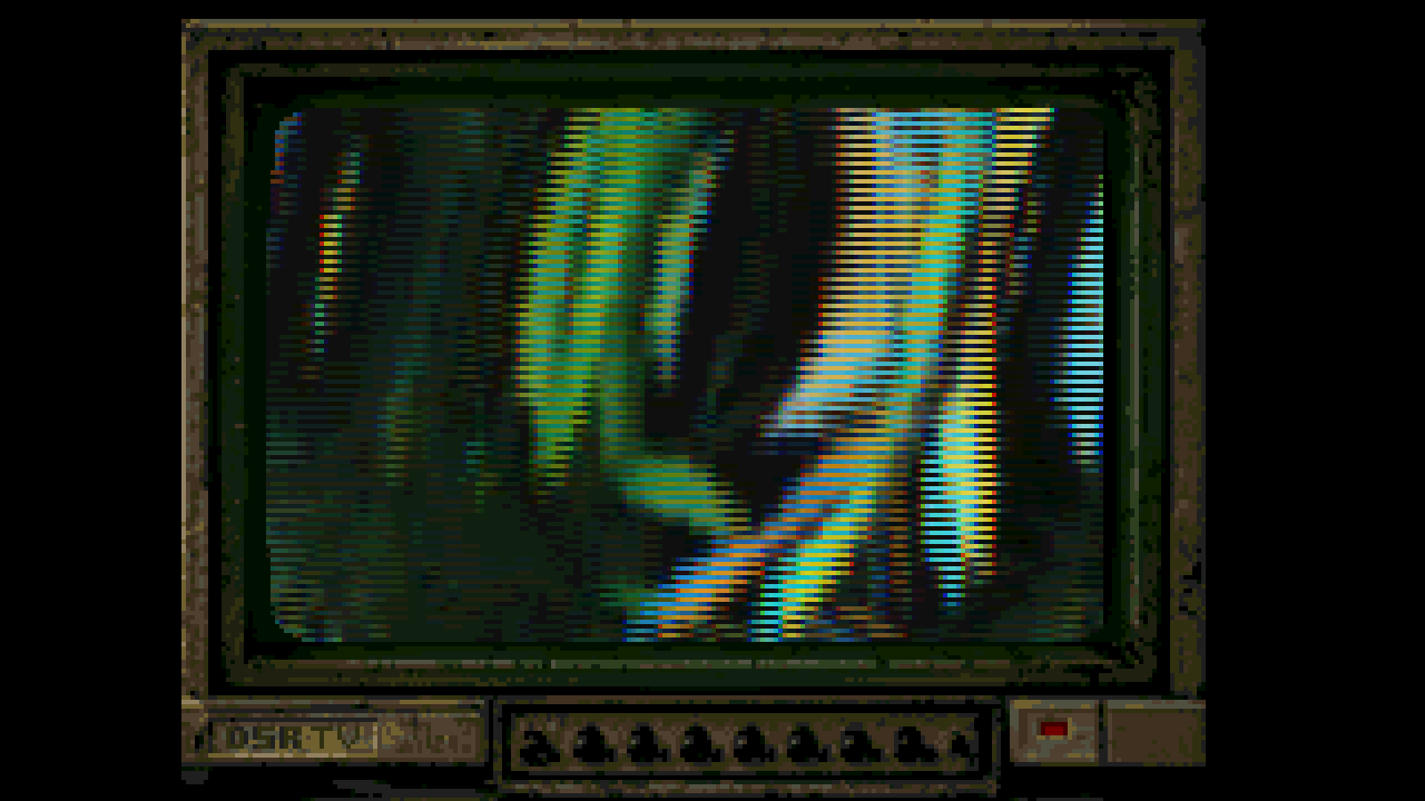
As if you hadn’t had enough of rotozoomers recently, I couldn’t resist shoehorning one more into this demo! No 4px columns here though, solid or otherwise. The flipped component scanline motion blur adds some more interest, along with the rubber distortion effect you get by adding a constant to the row delta. It was fun syncing the various parameters to the music too.
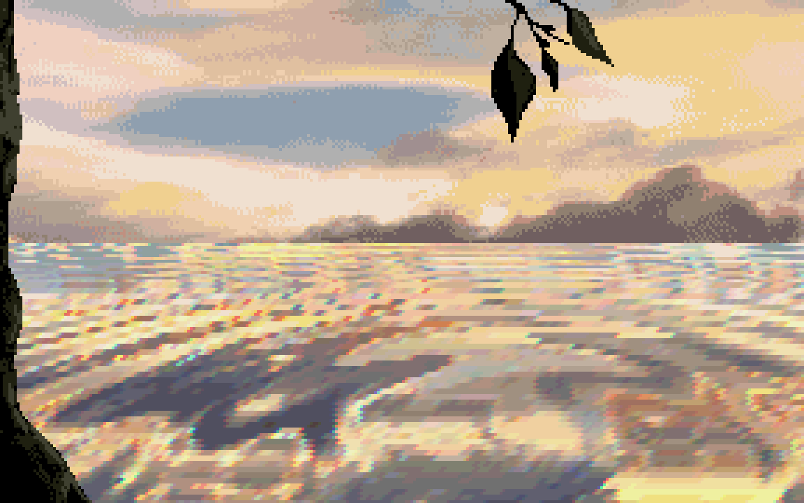
Sunrise #
This is a callback to the clouds part as we transition back to daytime. Most of the implementation is the same, but this time we include some foreground objects along with the horizon image. We had to make a compromise on the version to free up enough raster time for the next part to load. While the scrolling is still 50fps, the colours only update every other frame. This really isn’t noticeable, and I should have thought of it before!
Droplets #
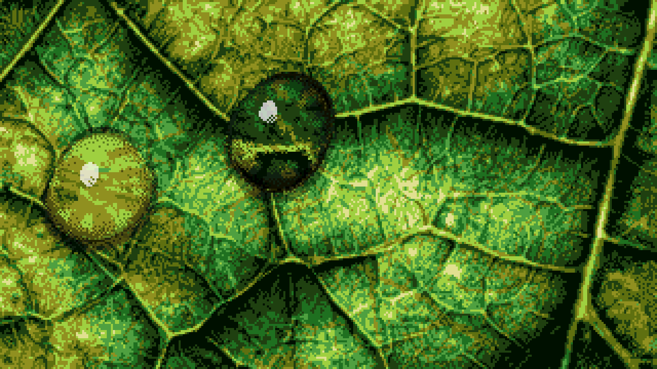
This effect is another one that came out of the question “how can we use 1x1 chunky effects in a way that don’t require drawing a full screen of pixels?”. It’s really two small table effects being blitted around the screen.
The key to making this look good was once again having good data. A simple sphere distortion wasn’t going to cut it. The droplets needed to be imperfect, and change shape as they move over the leaf. I needed to brush up on my Blender skills and make some wobbly animated droplet shapes. I applied an animated noise texture as the input for surface displacement, applied to a sphere. I rendered a range of animation frames with two different setups. One to get the UV offsets resulting from the object’s refraction properties, and one to get the tonal data.
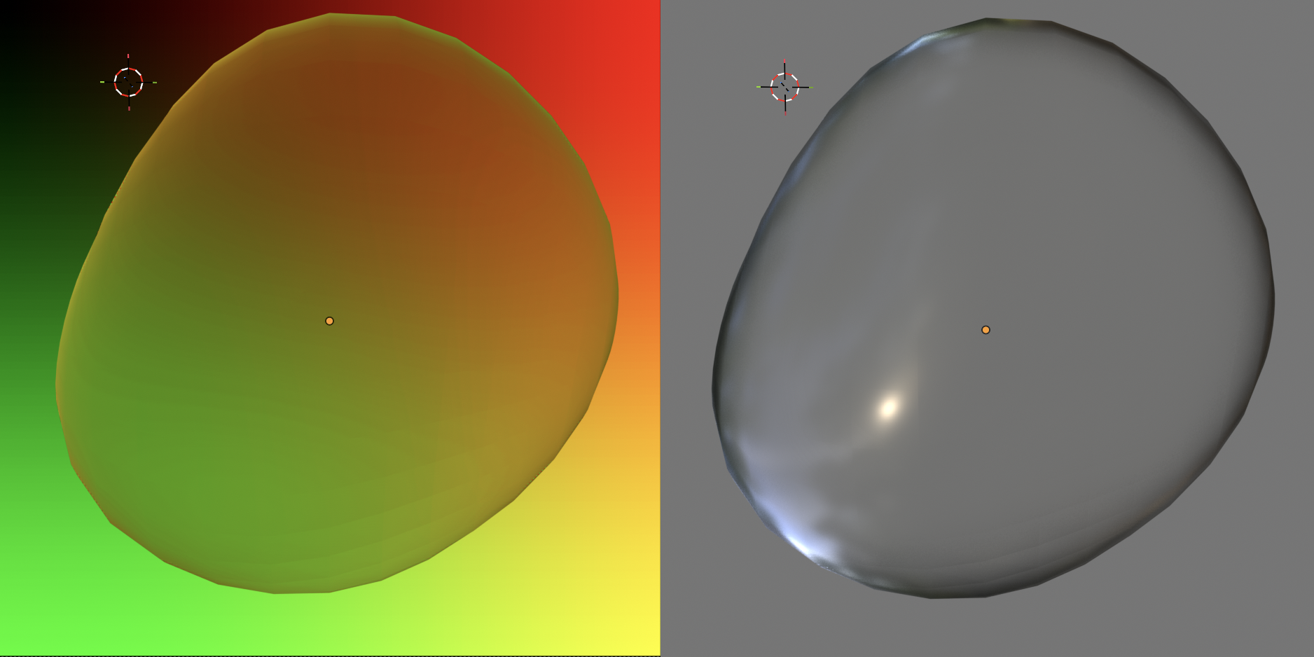
Blender scene setup for the two render modes
The tonal layer is converted to two bitplanes and blitted as regular bob on top of the three bitplane chunky output, using palette shifts to simulate lighting.
The path animation also needed to appear organic, with some speed variation and appearing to follow the curvature of the leaf. I used Catmull-Rom splines again and built a web based tool to edit them.
Water HAM #
For the penultimate part we have something that evolved out of the plasma effect we saw earlier.
Like the plasma, it uses a sum of a radial and linear sin wave, but the key differences are that the value is used as a relative offset into a 2D texture based on the sky image, rather than a linear palette, and the sin lookups have a perspective effect applied. Instead of the usual single cycle, the sin table repeats and decays, giving us the gradually dissipating waves. This means that the time between water drops is linked to the length of the table as it loops.
The sky uses a perspective scroll effect, where each line scrolls at a different speed, kind of like the floor in Street Fighter 2. The offset for each line is interpolated and translated into scroll and modulo values. This isn’t linked at all to the position of the texture in the “reflection”, but I think I get away with it!
The foreground objects are sprites. I rotoscoped the splash from a video reference, which was a fun process, and quite a bit of effort for a few frames of tiny 3 colour animation! Syncing the first drop fall to the music was the finishing touch that gave the effect its impact.
Butterfly #
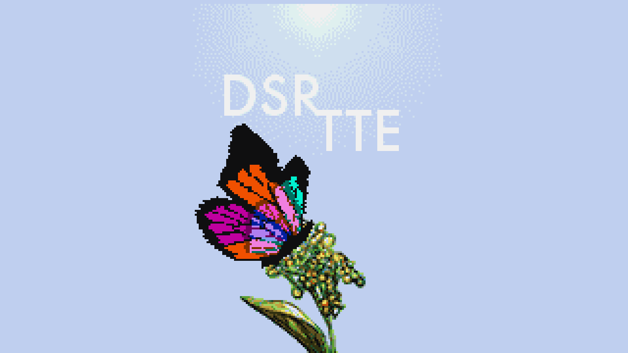
This final part barely made it in, and was party coded until after the deadline. I’m glad it did though, as I think it finishes things off nicely. Big thanks to Pellicus for delivering on this one.
In a couple of ways this is a callback to the start of the demo. The tech has a lot in common with the falling leaves part, and the flower is reused from the extended title screen. We wanted to end on a 1x1 texture mapped object, and in the back of my mind I had the TBL bird. I suppose a butterfly is a bit like an ultra-low poly bird, so it worked out pretty well!
Pellicus coded this part in C++, calling the existing C2P and texture mapper routines. The big idea for this was to get animation data from Unity, giving us a real timeline based editor allowing us to create realistic movement. Pellicus invested a huge amount of effort into the tooling for this, and we definitely didn’t take full advantage of the capabilities (yet!).
For various reasons, authoring the animation was left to Pellicus to do at the party, and although I’m sure he’d admit that this isn’t at the top of his skillset, we looked at lots of reference videos, and managed to get something pretty convincing.
Similar to the falling leaves, the wings are drawn to separate buffers in two bitplanes. The flower and text are sprites, which can also be controlled in the Unity tool. The wing transparency palette trick relies on a fair bit of artistic license. We did retrospectively find out that some transparent butterflies exist, but I don’t think any have asymmetric wing colours!
Conclusion #
So yeah, people seemed to like the demo, and we took first place. I’m really proud of what we achieved with this demo. It might not be everyone’s cup of tea, but it’s pretty close to the kind of demo we set out to make. Once again I got to work with a hugely talented group of people, and I think we created something that amounts to more than a sum of its parts. Of course there are things I would change, and things I wish we’d been able to include, but we have to save something for the next one!